Bayesian Network Modeling for University Admissions

Ever wondered if you’d get into your dream college? We all have been there and that’s why I (along with two other students from Habib University) we embarked on this exciting project: to build a system that uses Bayesian Networks to help students like you get a better idea of their chances of admission. If you don’t know, Bayesian Networks is a sub-field of AI. It is quite different from the mainstream “Deep-Nueral-Networks” which have become highly popular today. It is lesser known than neural networks but are more powerful than nueral networks for causal reasoning (Neural networks are bad at causal reasoning because cause and effect relationships are hardly captured in training data). A lot of experts believe that true AGI can be achieved only when we can make Bayesian Networks and Neural Networks work in harmony.

What’s the Goal?

Our project aims to give you a tool that can predict your likelihood of getting into different universities. You cannot totally rely on this tool, but we’re using data and a bit of clever math to help you make informed decisions about where to apply.

• The Big Picture: We’re not just looking at grades and test scores; we’re considering other factors too, like your extracurricular activities and whether you need financial aid.
• Personalized Predictions: Our system classifies universities into three categories for each student:
  • Reach Schools: Where your chances are lower.
  • Target Schools: Where you have a good shot.
  • Safety Schools: Where you’re likely to be admitted.
  • Currently, we’ve incorporated Reach and Target schools.

But why this can’t be done by Deep-Learning?

1. DNNs require lots of data, we simply don’t have that at our disposal
2. DNNs perform poorly on causal reasoning and college applications are highly complex, but can be captured through cause-and-effect relationships. However, we did use Llama 3.2 for scoring the extracurriculars, and we saw that such combination of different AI techniques made this problem solvable.

How Did We Do It? The Methodology Deep Dive 🤿

Here’s how we built our predictive system:

1. Data

• Common Dataset: We used the Common Dataset, a publicly available resource, to gather information about universities. Specifically, we used data from the 2021-2022, 2022-2023, and 2023-2024 academic years. We only used datasets for two universities since it was a manual process to intuitive convert raw data into conditional probabilities.
• What We Extracted:
  • Total applicants, acceptances, and enrollments, broken down by gender.
  • GPA and SAT score percentages for enrolled students.
  • Class rank divisions and financial aid awarded.
  • We calculated acceptance rates, financial aid rates, and how universities perceive high school academic standing and SAT scores.
• Choosing Our Universities: We focused on two schools for this project:
  • Harvard University as our Reach School.
  • University of Washington, Seattle as our Target School.
• To make our probabilities and network structure more accurate, we consulted two domain experts:
  • An admission officer from Habib University
  • A college counselor with experience working with both national and international students.
• These experts helped us understand the causal effects and impacts on the holistic college admission process.

2. Building the Bayesian Network 🕸️

A Bayesian Network is a cool way to represent how different factors influence each other, using probabilities. We used the GeNIe software for simulation.

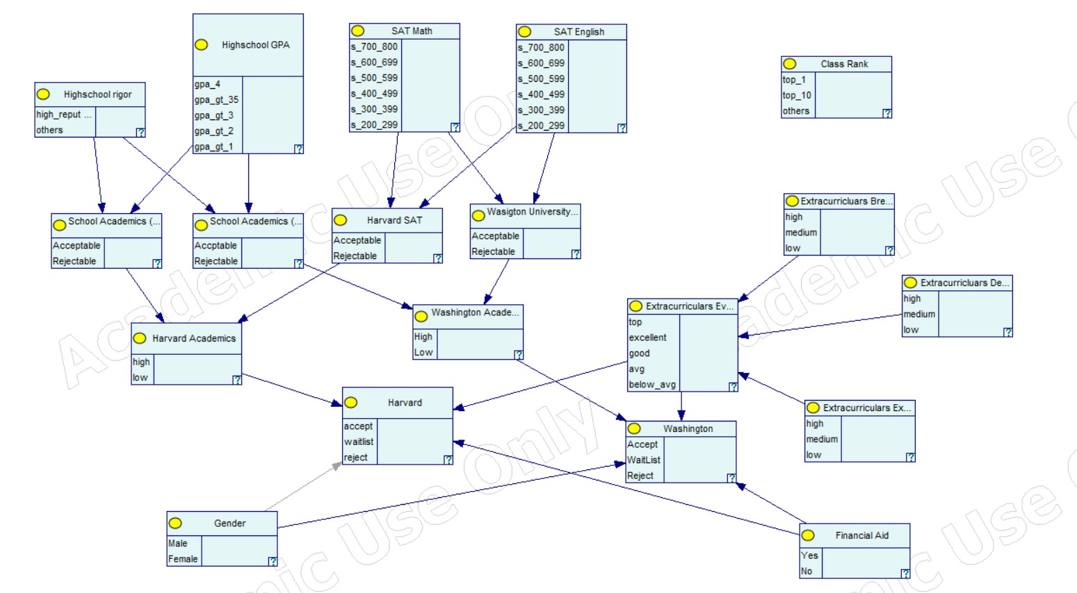Bayesian Network for the student admission process

• Nodes and Connections:
  • Universities are the leaf nodes.
  • We connected them to factors (nodes) that universities value, as stated in the Common Dataset.
  • For example, the Harvard node is connected to nodes for academic standing (based on their standards), gender, financial aid needs, and extracurricular activities.
• Parent-Child Relationships: We established relationships based on information from the Common Dataset; for example, Harvard considers SAT scores, GPA, rigor of high school coursework, and extracurriculars, but not class rank.
• Extracurriculars: We assessed extracurriculars based on depth (level of involvement), breadth (variety), and excellence (quality of performance).

We used Python’s PGMPy package to implement our Bayesian Network.

• Input Data: Users input their details, such as gender, financial aid needs, GPA, high school rigor, class rank, and SAT scores.
• LLM for Extracurriculars: We used a pre-trained LLama 3.2 3B model to evaluate extracurriculars based on breadth, depth, and excellence.
• Belief Propagation: We then used belief propagation to calculate the probability of admission.

5. Testing and Evaluation 🤔

• Benchmarking: We tested our network by comparing its predictions to those from CollegeVine, an online platform that also predicts admission chances.
• Random Profiles: We generated 26 random student profiles on CollegeVine and compared CollegeVine’s predictions with our network’s output.
• The Results: Our overall accuracy was 64%.
  • Our Mean Absolute Error (MAE) was 8.16 for Harvard and 21.68 for the University of Washington.
  • Our model’s distributions followed a similar pattern to CollegeVine’s, but there were some differences in the densities as shown below

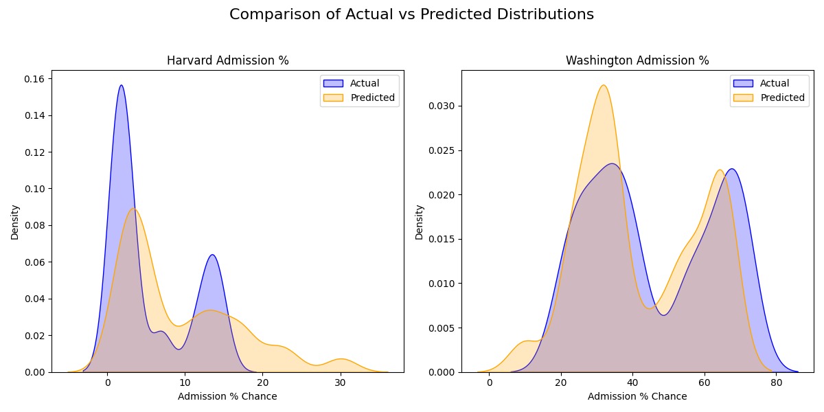Distribution of the Actual vs Predicted values

Causal Inference: More Than Just Numbers! 🤯

One of the most fascinating parts of this project was how well our Bayesian model captured causal relationships. Even though our overall accuracy wasn’t super high, the logical inferences were spot-on.

• Logic in Action: For example, if a student had a high chance of getting into Harvard, our model correctly increased the probability of them getting into the University of Washington.
  • Being accepted at the University of Washington did not improve the chances of admission to Harvard.
  • High SAT scores that were acceptable for Harvard also increased the acceptability for the University of Washington.
• Key Factors: We found that GPA and SAT scores had the biggest impact on admission chances. Gender didn’t play a role, but interestingly, students who didn’t request financial aid saw a slight boost in their chances. Additionally, diversity in extracurriculars also helped.

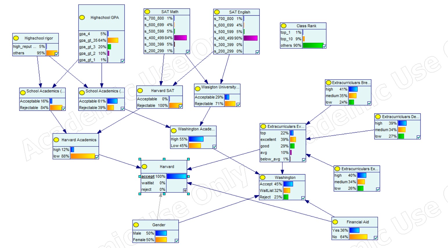Evidence on the Harvard Node, accpeting admission

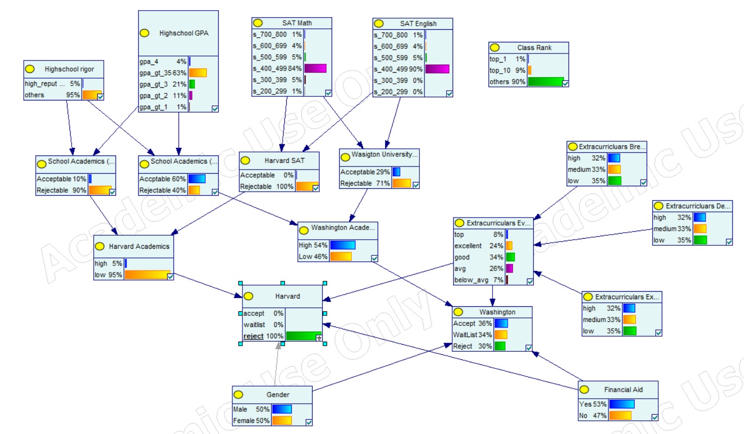Evidence on the Harvard Node, rejecting admission

Running the Project Yourself

Option 1: The Django App

Our project is a Django application, which means it has a user interface where you can input your data and get predictions.

• Django Tutorial: If you’re new to Django, check out the official tutorial [external link to Django tutorial].
• Note: You don’t need Django for the core functionality, which is the Bayesian network.

Option 2: The GeNIe Graphical Model

• GeNIe Software: You can use the GeNIe software to graphically run the network.
• Network.xdsl File: You’ll need to use the Network.xdsl file (a file format used in GeNIe). This file contains the structure and parameters of our Bayesian network.
• Manual Input: In GeNIe, you can manually input data (like the ones described in the python application) to view the probabilities.

Code Snippets: A Peek Under the Hood ⚙️

Let’s look at some of the key parts of our Python code (found in model.py.txt.txt):

1. Defining the Bayesian Network Structure:

   from pgmpy.models import BayesianNetwork
   noisy_or = BayesianNetwork([
       ('Extracurriculars Depth', 'Extracurriculars Evaluation'),
       ('Extracurriculars Breadth', 'Extracurriculars Evaluation'),
       ('Extracurriculars Excellence', 'Extracurriculars Evaluation'),
       ('Highschool rigor', 'School Academics Harvard'),
       ('Highschool GPA', 'School Academics Harvard'),
       # truncated code (other edges)
   ])
   

   We use the pgmpy.models.BayesianNetwork class to define the nodes and connections in our network. For example, ('Extracurriculars Depth', 'Extracurriculars Evaluation') indicates that ‘Extracurriculars Depth’ influences ‘Extracurriculars Evaluation’.

2. Defining Conditional Probability Distributions (CPDs):

   from pgmpy.factors.discrete import TabularCPD
   
   cpd_gender = TabularCPD(variable='Gender', variable_card=2,
   values=[[0.5], [0.5]],
   state_names={'Gender': ['Male', 'Female']})
   

   Here, we define a CPD for ‘Gender’, which has two states: ‘Male’ and ‘Female’, each with a probability of 0.5.

   cpd_highschool_gpa = TabularCPD(variable='Highschool GPA', variable_card=5,
   values=[[0.1], [0.2], [0.3], [0.2], [0.2]],
   state_names={'Highschool GPA': ['4', '3.5', '3', '2', '1']})
   

   The CPD for Highschool GPA shows that we have five categories of GPA with a distribution of probabilities assigned to each of them.

3. Noisy-OR Implementation:

   cpd_extracurriculars_evaluation = TabularCPD(variable='Extracurriculars Evaluation', variable_card=5,
       values=[
           [0.2]*27,
           [0.2]*27,
           [0.2]*27,
           [0.2]*27,
           [0.2]*27
       ],
       evidence=['Extracurriculars Depth', 'Extracurriculars Breadth', 'Extracurriculars Excellence'],
       evidence_card=,
       state_names={
       'Extracurriculars Depth': ['High', 'Medium', 'Low'],
       'Extracurriculars Breadth': ['High', 'Medium', 'Low'],
       'Extracurriculars Excellence': ['High', 'Medium', 'Low'],
       'Extracurriculars Evaluation': ['Top', 'Excellent', 'Good', 'Average', 'Poor']
       })
   

   This shows an example of an implementation of a noisy-OR gate which determines that extracurricular evaluation will be an average of 0.2 for each category of evaluation considering the three types of extracurricular attributes.

4. Conditional Probability of SAT Scores:

   cpd_harvard_sat = TabularCPD(variable='Harvard SAT', variable_card=2,
       values=[
           [0.8645, 0.07969999999999999, 0.00592, 0.00095, 0.00095, 0.00095, 0.045, 0.00413, 0.000306, 0.00049, 0.00049, 0.00049, 0.0006643, 0.0000614, 0.000006, 0, 0, 0, 0.00091, 0.000084, 0, 0, 0, 0, 0.00091, 0.000084, 0, 0, 0, 0, 0.00091, 0.000084, 0, 0, 0, 0],
           [0.1355, 0.9203, 0.99408, 0.99905, 0.99905, 0.99905, 0.955, 0.99587, 0.999694, 0.9999508, 0.9999508, 0.9999508, 0.9993357, 0.9999388, 0.9999955, 1, 1, 1, 0.99909, 0.999916, 1, 1, 1, 1, 0.99909, 0.999916, 1, 1, 1, 1, 0.99909, 0.999916, 1, 1, 1, 1]
       ],
       evidence=['SAT Math', 'SAT English'],
       evidence_card=,
       state_names={
       'SAT Math': ['700-800', '600-699', '500-599', '400-499', '300-399', '200-299'],
       'SAT English': ['700-800', '600-699', '500-599', '400-499', '300-399', '200-299'],
       'Harvard SAT': ['High', 'Low']
       })
   

   This defines the conditional probability of a node Harvard SAT being high or low, given the combination of the SAT English scores and SAT Math scores using a truth table.

5. Making Queries

   from pgmpy.inference import BeliefPropagation
   inference = BeliefPropagation(noisy_or)
   
   for uni in ['Harvard', 'Washington University']:
       query_result = inference.query(variables=[uni])
       print(query_result.values)
   

   We use pgmpy.inference.BeliefPropagation to make probability queries about the network and see the initial probabilities.

   inference = BeliefPropagation(noisy_or)
   for uni in ['Harvard', 'Washington University']:
       query_result = inference.query(variables=[uni], evidence={
           'Gender': 'Female',
           'Financial Aid': 'No',
           'Highschool GPA': '4',
       })
   print(query_result.values)
   

   Then, we make queries using some evidence on the nodes of the network like gender, financial aid needs, and highschool GPA for a given university to evaluate changes in the probability.

Limitations and Future Steps 🚧

Like all projects, ours has some limitations:

• Our model initially struggled with mid-tier universities because their acceptance probabilities for high SAT scores were lower than expected. We had to use prior probabilities to compensate this.
• We may not have considered all factors that universities use in the admission process (like AP honors courses).
• Our model doesn’t fully utilize the class rank factor because our chosen universities didn’t consider it.
• We need more test data to get more accurate results.

Conclusion 🎉

Bayesian Networks can be a powerful tool for predictive reasoning where there is less data and causal relationships are important. Even though we faced some limitations, Our model is effective at capturing causal inferences and and we may extend it in the future.